本案例有关说明
- 本案例是分布拟合检验预测、单因素方差分析One-Way ANOVA的基础前导篇。基本概念不在此赘述。
- 本案例分析所用数据为“19财管管理会计成绩.xlsx”。
- 该数据可以在我的百度网盘上*载下**。
链接:https://pan.baidu.com/s/1ARmBISe_xask-qqaNyaM1A
提取码:qa0f
- 本案例为本人学习笔记,数据及分析结论供学习和教学参考之用。
描述性统计基本认识
描述性统计,是指通过数据计算“统计量”用来描述数据特征的活动。描述性统计分析主要包括以下几个方面的分析:
- 频数分析
- 集中趋势分析
- 离散程度分析
- 数据分布
- 绘制统计图
引入需要使用到的库
import pandas as pd
import numpy as np
import matplotlib.pyplot as plt
import seaborn as sns
这个引入库的动作,是首先要做的。

read_excel()读入待分析数据
df = pd.read_excel('19财管管理会计成绩.xlsx',sheet_name='19财管管理会计')
数据集:"19财管管理会计成绩.xlsx",两列,class为分类变量,glkj为可度量变量。
- class:班级。19财管1—19财管6。分类变量。
- glkj:管理会计,该科目考试成绩。

Descriptive Statistics
# 分组聚合,统计均值、次数、标准差等
stats = df.groupby('class')['glkj'].agg(['mean', 'count', 'std','min','max'])
# 计算0.05水平下的置信区间
ci95_hi = []
ci95_lo = []
co_v = []
for i in stats.index:
m, c, s = stats.loc[i,['mean','count','std']]
ci95_hi.append(m + 1.96 * s/math.sqrt(c))
ci95_lo.append(m - 1.96 * s/math.sqrt(c))
co_v.append(s/m)
stats['ci95_LB'] = ci95_lo
stats['ci95_UB'] = ci95_hi
stats['c.v'] = co_v
统计量stats
- mean:均值std : 标准差min/max : 最小/最大值
- median : 中位数
- skew : 偏度
- ci : 置信区间
- c.v : 变异系数
上述“统计量”的基本概念计算方法及计算公式网上讲解很多,在此就不具体列出了,需要的请百度。
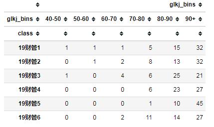
统计量如下图所示:


上面图表反映的基本信息
- 管理会计科目成绩平均值都较高,中位数均在90分以上的有四个班,特别是19财管5班均值高达93分,中位数95分。该班成绩离散程度最小,成绩变异程度最小。
- 所有班级管理会计科目成绩分布呈现“左偏”。均值小于中位数。
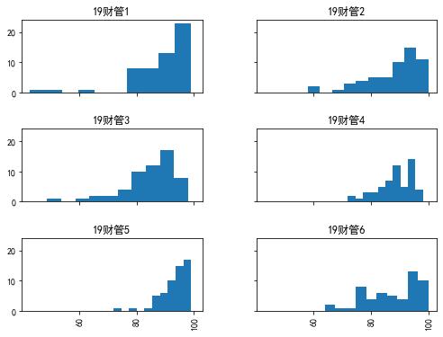
boxplot & hist:了解大概的分布、发现异常值
# Draw a nested boxplot
df.boxplot(column='glkj', by='class', grid=False)
sns.hist(column='glkj', by='class',figsize=(8,6) ,sharex=True,sharey=True)
sns.despine(offset=10, trim=True)

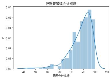
核密度kde: 了解分布形态
#use sys default settings
ax = sns.distplot(a= df['glkj'])
ax.set(title='19财管管理会计成绩', xlabel='管理会计成绩',ylabel='P')
- Signature:
sns.distplot(a, bins=None, hist=True, kde=True)
该图的成绩分段使用系统默认的设置。结果整体成绩是否为“左偏”?确实是“左偏”。
总体成绩的hist & kde:了解总体分布情况
# set bins
fig,(ax1,ax2)= plt.subplots(1,2,sharex=True, figsize=(7,5))
plt.subplot(1,2,1)
ax1 = sns.distplot(a=df['glkj'], bins=[10, 20, 30, 40, 50, 60, 70, 80, 90,100],
norm_hist= False,hist=True, kde=False,label='管理会计成绩')
ax1.set(title='19财管管理会计成绩',xlabel='管理会计成绩',ylabel='Count')
ax1.legend(loc='best')
#plt.tight_layout(rect=(1, 1, 1, 1)) #设置默认的间距
plt.subplot(1,2,2)
ax2 = sns.distplot(a=df['glkj'], bins=[10, 20, 30, 40, 50, 60, 70, 80, 90,100],
norm_hist= True,hist=True, kde=True,label='管理会计成绩KDE',color='green')
ax2.set(title='19财管管理会计成绩KED',xlabel='管理会计成绩',ylabel='P')
ax2.legend(loc='best')
plt.subplots_adjust(wspace=0.3)
plt.show()

使用pd.cut():自定义分段及频数统计
bins = [0, 10, 20, 30, 40, 50, 60, 70, 80, 90, 101]
labels = ['0-10','10-20','20-30','30-40','40-50','50-60','60-70','70-80','80-90','90+']
- x:需要切分的数据
- bins:切分区域
- right : 是否包含右端点默认True,包含
- labels:对应标签,用标记来代替返回的bins,若不在该序列中,则返回NaN
- retbins:是否返回间距bins
- precision:精度
- include_lowest:是否包含左端点,默认False,不包含
- right : 是否包含右端点默认True,包含。该例为不包括False。[a,b)
df['glkj_bins'] = pd.cut(df['glkj'], bins=bins, labels=labels, include_lowest=True, right=False)
class_count = df.groupby(by= 'class')['glkj_bins'].value_counts()
pd_class_count= pd.DataFrame(class_count)
pd_unstack = pd_class_count.unstack(fill_value=0)
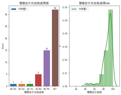
分班级hist、kde:了解各班分布情况
for i in range(6):
fig,(ax1,ax2)= plt.subplots(1,2,sharex=True,figsize=(8,6))
plt.subplot(1,2,1)
ax1 = sns.barplot(count_bins,pd_unstack.values[i],label=pd_unstack.index[i])
ax1.legend(loc='best')
ax1.set(xlabel= '管理会计分段成绩',ylabel= 'Count',title = '管理会计分班级成绩图')
list_n = pd_unstack.values[i]
for j, txt in enumerate(list_n):
ax1.annotate(txt, (j, list_n[j]+0.6),horizontalalignment='center',verticalalignment='center')
plt.subplot(1,2,2)
ax2 = sns.distplot(a=df.loc[df['class']== pd_unstack.index[i]]['glkj'],bins=[10, 20, 30, 40, 50, 60, 70, 80, 90,100],norm_hist= True,hist=True, kde=True,label= pd_unstack.index[i],color='green')
ax2.set(title='管理会计分班级成绩kde',xlabel='管理会计成绩',ylabel='P')
ax2.legend(loc='best')
plt.show()