作者:slan
地图制作是地理空间数据的可视化的一种方式。为了确保视觉效果与它们所基于的数据准确一致,它试图以一种非技术性又受众更容易理解和解释的形式来表达数据。无论你哪里得到的数据,当它被绘制成地图以更直接地方式来描述它所指的地点时,它将更有影响力。
1. 介绍
首先我们先了解,地理空间数据可视化的基本地图类型大概可以分为:
point Map(点式地图)、Proportional symbol map(比例符号地图)、cluster map(集群地图)、choropleth map(等值区域图)、cartogram map(变形地图)、hexagonal binning map(六边形分箱图)、heat map(热力图)、topographic map(地形图)、flow map(流向图)、spider-map (蛛状图)、Time-space distribution map(时空分布图)、data space distribution map(数据空间分布图)等。
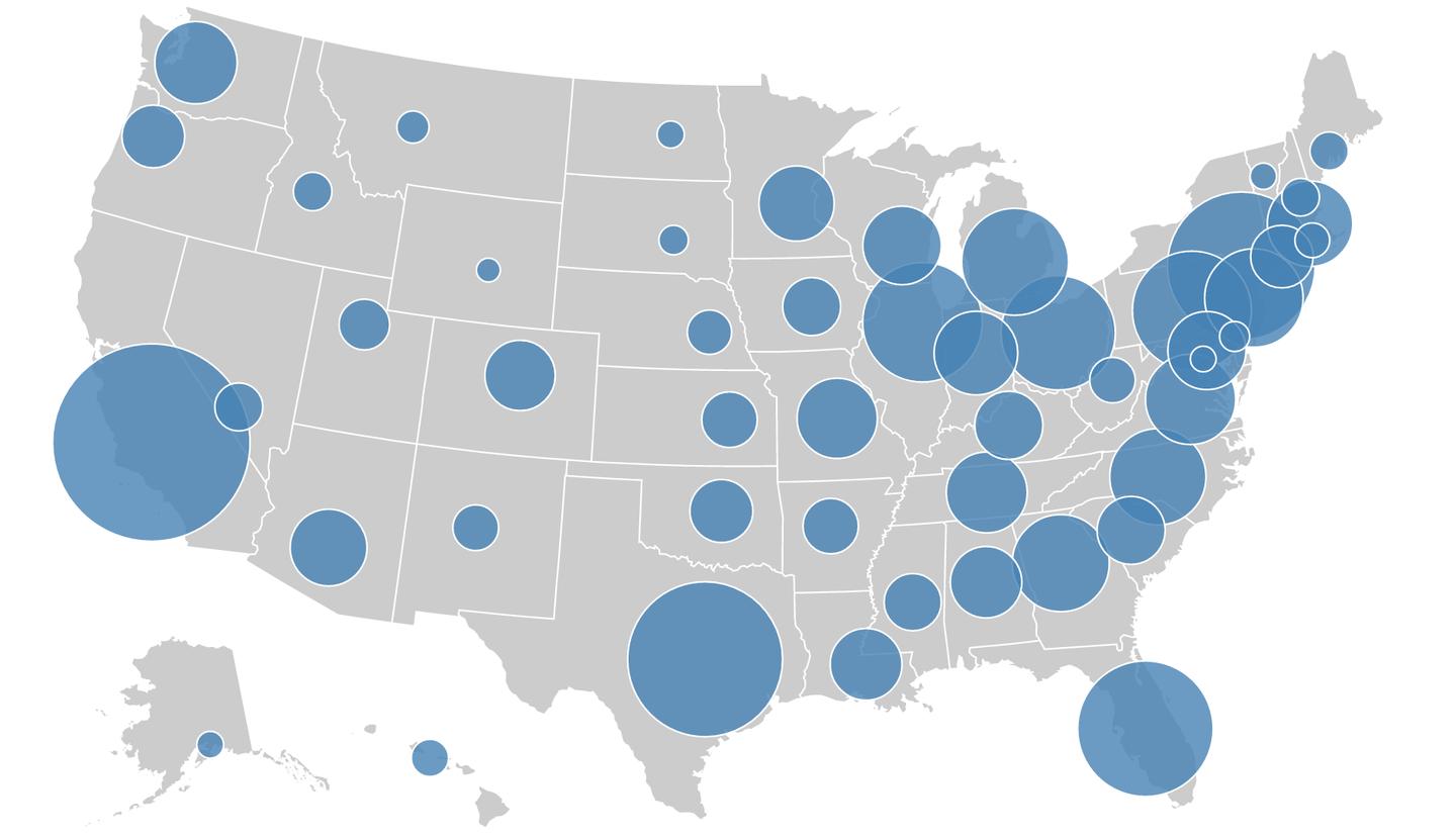
本文主要介绍如何绘制 Proportional symbol map(比例符号地图) ,比例符号图是点地图的一个变体。它使用大小不同的地图符号来表示一个定量的变量(通常是圆形),如图所示。
本文目的是用一个 Python 程序为给定的一个多边形 shapefile 和一个定量属性,绘制一个比例点符号地图。该地图会包括显示多边形的基础地图和点符号。
2. 导入包
首先导入 numpy 和 matplotlib 包。在下面导入的包中,numpy 对于这个项目不是必需的,但是它可以通过在数组级别上进行计算而不是使用循环来引入更高的性能。
import numpy as np
import matplotlib.pyplot as plt
from matplotlib.path import Path
from matplotlib.patches import PathPatch
from geom.shapex import *
from geom.point import *
from geom.point_in_polygon import *
from geom.centroid import *
注意:目标路径“geom”已经存在,并且不是空目录,请解压我链接中的文件保存到本地导入。
链接: python - 腾讯 iWiki (woa.com)
3. 数据处理过程
3.1. 获取多边形和属性
找到上面链接的 uscnty48area 文件*载下**解压到本地
fname = 'C:/Users/Tencent_Go/Desktop/python/area/uscnty48area.shp'
mapdata = shapex(fname)
print(f"The number of regions: {len(mapdata)}")
然后我们可以看到 regions 的数量为:3109
然后我们看一下列表 mapdata 中字典的数据结构。我们将使用递归函数输出字典中的所有键。
def print_all_keys(dic: dict, k=None, spaces=0):
"""这个函数将打印出字典中的所有键,以及子字典中的所有键。"""
    ks = dic.keys()  # 得到了所有的键

    # 打印一个标题来表明这是哪个字典:
    if k is None:
# 这是字典的基本情况。
        print("All keys:")
else:
# 这是我们字典的子字典
        print("-" * spaces * 4 + f"Keys in sub-dictionary '{k}':")
# 打印所有键
    print("-" * spaces * 4 + f"{[key for key in ks]}\n")

    spaces += 1
    for k in ks:
# 遍历所有键,检查某个键是否指向子字典
        if type(dic[k]) == dict:
# 如果存在子字典,则再次调用该函数
            print_all_keys(dic[k], k, spaces)

print_all_keys(mapdata[0])
All keys: ['type', 'geometry', 'properties', 'id']
----Keys in sub-dictionary 'geometry': ----['type', 'coordinates']
----Keys in sub-dictionary 'properties': ----['NAME', 'STATE_NAME', 'FIPS', 'UrbanPop', 'Area', 'AreaKM2', 'GEO_ID', 'PopDensity']
我们看看 shapex 文件中的一个字典示例
display(mapdata[1])
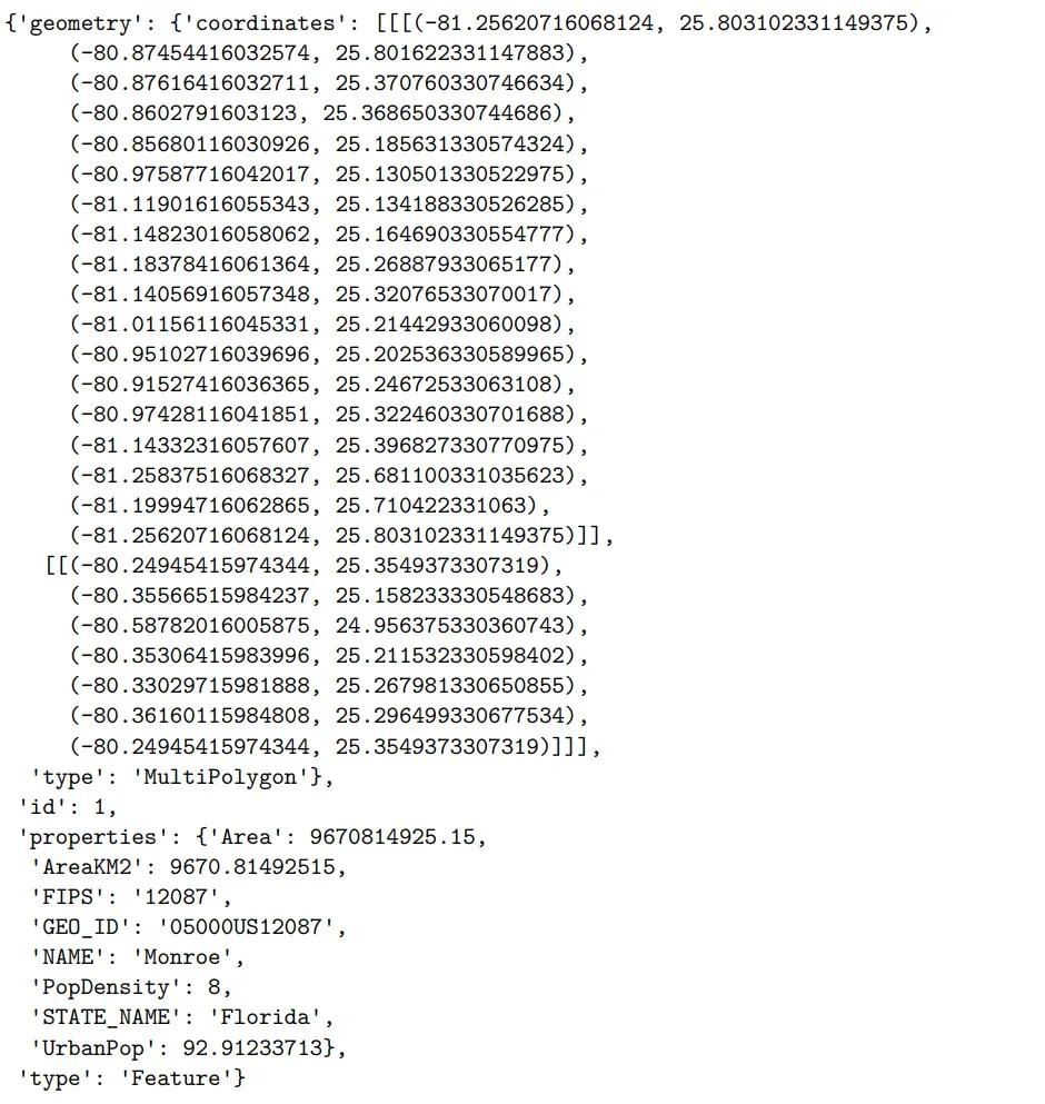
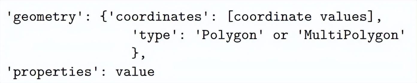
为了正确处理数据并得到所需的比例点符号图,请确保输入的 shapex 文件是以下结构
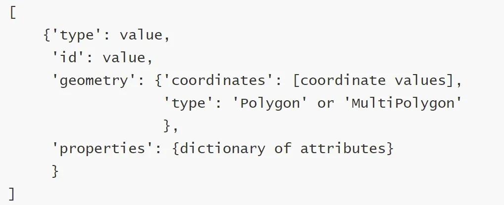
如果不是这样,文件至少要包含下面两个部分
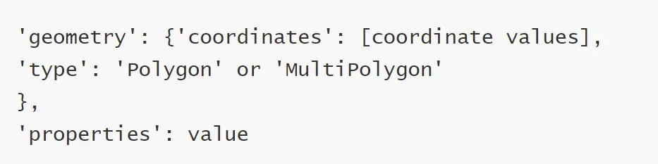
其他结构会在处理过程中引起 keyerror。我们可以通过下面的函数指出我们需要的键来使它更灵活地接受不同格式的字典,但这将显著的增加工作负载,这不是本文的目的。我们将首先创建一个函数来从 shapex 对象中提取我们需要的信息。函数的逻辑和过程将在函数中讨论。
def get_coordinates_features(mapdata, attribute=None, verbose=False):
"""
这个函数将一个地图数据作为输入,并提取坐标,得到数据中所有多边形和组合多边形的属性(如果有指定)。
属性的返回列表与多边形/组合多边形的坐标的返回列表相同
输入:
Mapdata:一个shapex类对象或一个字典列表。
Attribute: mapdata中属性的名称。
Verbose:是否打印信息。
输出:
polygons:所有多边形的坐标列表。
multipolygons:所有组合多边形的坐标列表。
Attribute_poly:所有多边形属性值的列表。
Attribute_multipoly:与所有组合多边形的相似性。
X_min, x_max, y_min, y_max: x和y坐标的最小值和最大值。
"""
# 初始化我们所需要的输出
polygons = []
multipolygons = []
attribute_poly = []
attribute_multipoly = []
regions = []
# 这可能因数据而异
x_min = 500
x_max = -500
y_min = 500
y_max = -500
# 检查我们是否按要求拥有有效的属性
if attribute is None:
print('No attribute is selected, please specify manually afterwards.')
elif attribute not in mapdata[0]['properties'] and attribute is not None:
print('The attribute selected is not in the first data, please check and select another!')
else:
print(f"'{attribute}' selected as the attribute.")
# 遍历mapdata,每个元素都是代表一个区域的
for i in range(len(mapdata)):
"""
注意:我们将把多边形和组合多边形分开,是因为它们具有不同的结构。
每个组合多边形都是由多个多边形组成的列表,但它们在地理数据的意义上是不可分离的。
"""
if mapdata[i]['geometry']['type'].lower() == 'polygon':
# 如果有,则附加必要的属性。
if attribute in mapdata[i]['properties']:
attr = mapdata[i]['properties'][attribute]
attribute_poly.append(attr)
else:
attribute_poly.append(None)
# 得到坐标的列表,转换成多边形附加上
coodi = mapdata[i]['geometry']['coordinates'][0]
polygon = [Point(p[0], p[1]) for p in coodi]
polygons.append(polygon)
# 更新x y 的最小值和最大值坐标
coodi_x = [p[0] for p in coodi]
coodi_y = [p[1] for p in coodi]
if min(coodi_x) < x_min:
x_min = min(coodi_x)
if max(coodi_x) > x_max:
x_max = max(coodi_x)
if min(coodi_y) < y_min:
y_min = min(coodi_y)
if max(coodi_y) > y_max:
y_max = max(coodi_y)
# 如果我们想打印信息(前面注释写道)
if verbose:
city = mapdata[i]['properties']['NAME']
state = mapdata[i]['properties']['STATE_NAME']
regions.append(city, state)
print(f"Polygon appended: {city}, {state}")
elif mapdata[i]['geometry']['type'].lower() == 'multipolygon':
# 对于组合多边形,我们需要额外的循环
# 如果有需要,我们追加必须的属性
if attribute in mapdata[i]['properties']:
attr = mapdata[i]['properties'][attribute]
attribute_multipoly.append(attr)
else:
attribute_multipoly.append(None)
# 初始化一个列表来收集组合多边形
multipolygon = []
coodis = mapdata[i]['geometry']['coordinates'] # 坐标列表
for j in range(len(mapdata[i]['geometry']['coordinates'])):
# 循环遍历所有多边形,转换并追加到集合
coodi = coodis[j][0]
polygon = [Point(p[0], p[1]) for p in coodi]
multipolygon.append(polygon)
# 更新x y 的最小值和最大值坐标
coodi_x = [p[0] for p in coodi]
coodi_y = [p[1] for p in coodi]
if min(coodi_x) < x_min:
x_min = min(coodi_x)
if max(coodi_x) > x_max:
x_max = max(coodi_x)
if min(coodi_y) < y_min:
y_min = min(coodi_y)
if max(coodi_y) > y_max:
y_max = max(coodi_y)
# 将多边形集合附加到组合多边形列表。
multipolygons.append(multipolygon)
# 如果我们想打印信息
if verbose:
city = mapdata[i]['properties']['NAME']
state = mapdata[i]['properties']['STATE_NAME']
regions.append(city, state)
print(f"MultiPolygon appended: {city}, {state}")
else:
# 如果没有多边形或组合多边形,跳转到下一个循环。
print(f"Make sure it is a polygon shape file for {i}th county.")
continue
# 打印摘要并返回
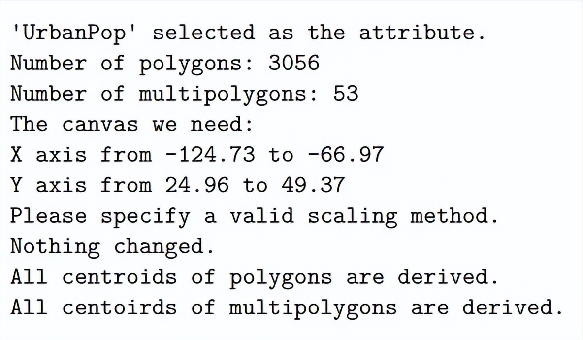
print(f"Number of polygons: {len(polygons)}")
print(f"Number of multipolygons: {len(multipolygons)}")
print(f"The canvas we need: ")
print(f"X axis from {round(x_min, 2)} to {round(x_max, 2)}")
print(f"Y axis from {round(y_min, 2)} to {round(y_max, 2)}")
return polygons, multipolygons, attribute_poly, attribute_multipoly, \
regions, x_min, x_max, y_min, y_max
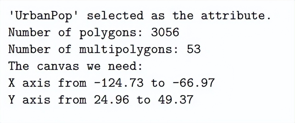
让我们测试函数,并获得进一步处理所需的数据格式。
该函数可以返回城市和州的列表,以便在图形中提供额外的文本,或者匹配来自其他数据源的自定义属性。
我将 regions.append()方法保留在verbose (详细信息)中,因为我可以在其他国家的数据中想象到这一点。对于其他国家的数据源,可能没有 state (州),从而导致 KeyError 。 因此,在这种情况下,对于该数据,我们可以简单地关闭 verbose。必须有一个更灵活的方法来指定,我们想在函数参数中返回哪些键,但这已经超出了本文的目的范围。
polygons, multipolygons, attribute_poly, attribute_multipoly, \
regions, x_min, x_max, y_min, y_max = get_coordinates_features(mapdata,
                                                                   attribute='UrbanPop', verbose=False)
3.2. 变化量化属性
在这一部分,我们需要缩放属性,以便在最终的图形中具有比例符号。我遵循了 维基百科 中介绍的三种比例缩放方法,并加入了一个简单的乘数:
1. Absolute Scaling(绝对量表法)
图中任意两个数值属性的面积应该与这两个属性的值具有相同的比例。从形式上看,它会是这样的:


这是我们比例所有属性所需要的关系。
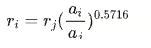
2. Apparent Magnitute (Flannery) Scaling(表观方法缩放法)
这种方法是基于心理物理的詹姆斯·弗兰纳里在 1956 年做的实验。他指出这种方法使人更容易认识到关系的大小。缩放公式如下:
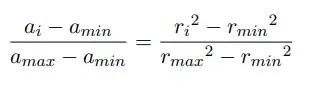
3. Interpolated Scaling(插值缩放法)
前两种方法的主要问题是,如果值的数量大小比较大,而它们之间的差异相对较小,则很难区分其点本身。例如,对于从 1 到 10 的值,我们可能会看到不同大小的符号,但是对于从 10000 到 11000 的值,我们可能会看到相似的圆圈。该方法将把范围“扩展”到我们需要的最小值和最大值。这个关系遵循:
4. Simple Multiplier(单纯形乘数法)
属性将简单地乘以一个数字。
在下面的函数中,我们可以为图上的圆指定我们想要的最大半径和最小半径(仅用于插值缩放)。所有属性的值将根据我们选择的方法和半径进行相应的调整。
def attribute_scaling(attribute_poly, attribute_multipoly,
                      max_radius=100, min_radius=1, multiplier=100,
                      scale='absolute'):
"""
    方法可以在这里找到:Proportional symbol map - Wikipedia
    该函数将多边形和组合多边形的属性作为输入并使用我们指定的方法和半径缩放它们。

    输入:
    Attribute_poly:所有多边形的属性列表
    Attribute_multipoly:所有组合多边形的属性列表
    Max_radius:我们想要的最大圆的半径
    Min_radius:我们想要的最小圆的半径。
               它只会在插入比例方法时使用
               应该是一个介于0和max_radius之间的值。
    multiplier:为简单乘数法。
    Scale:缩放法

    输出:
    缩放attribute_poly和attribute_multipoly
    """

    # 如果比例不可识别或输入的min_radiu无效,则不要缩放
    if scale not in ['absolute', 'flannery', 'interpolated', 'multiplier']:
print('Please specify a valid scaling method.\nNothing changed.')
return attribute_poly, attribute_multipoly

if scale == 'interpolaed' and (min_radius is None or
                                   min_radius <= 0 or
                                   min_radius >= max_radius):
print('Please specify a valid min_radius between 0 and max_radius.\nNothing changed.')
return attribute_poly, attribute_multipoly

# 获取属性的最大值,这是缩放的基线
    attr_max = max(max(attribute_poly), max(attribute_multipoly))

# 基于最大值缩放/转换属性
    if scale == 'absolute':
        attribute_poly = [np.sqrt(a / attr_max) * max_radius for a in
                          attribute_poly]
        attribute_multipoly = [np.sqrt(a / attr_max) * max_radius for a in
                               attribute_multipoly]
print('Absolute scaling applied.')

elif scale == 'flannery':
        attribute_poly = [(a / attr_max) ** 0.5716 * max_radius for a in
                          attribute_poly]
        attribute_multipoly = [(a / attr_max) ** 0.5716 * max_radius for a in
                               attribute_multipoly]
print('Apparent magnitude (Flannery) scaling applied.')

elif scale == 'interpolated':
"""
        interpolated 是最小-最大-缩放
        获取属性的最小值
        它将乘以0.99,因为地图上最小的属性需要至少一个点,否则它的半径将为0
        如果数据中没有值也没有影响,将不会为其呈现标识。
        """
        attr_min = min(min(attribute_poly), min(attribute_multipoly)) * 0.99
        attribute_poly = [np.sqrt((a - attr_min) /
                                  (attr_max - attr_min) *
                                  (max_radius ** 2 - min_radius ** 2) +
                                  min_radius ** 2
                                  ) for a in attribute_poly]
        attribute_multipoly = [np.sqrt((a - attr_min) /
                                       (attr_max - attr_min) *
                                       (max_radius ** 2 - min_radius ** 2) +
                                       min_radius ** 2
                                       ) for a in attribute_multipoly]
print(f'Interpolated scaling applied: from {min_radius} to {max_radius}.')

elif scale == 'multiplier':
if multiplier <= 0:
print('Please specify a valid multiplier.\nNothing changed.')
return attribute_poly, attribute_multipoly
else:
            attribute_poly = [multiplier * a for a in attribute_poly]
            attribute_multipoly = [multiplier * a for a in attribute_multipoly]
print(f'Multiplier scaling applied: {multiplier}x.')

else:
# 更多的方法可以被添加
        # 只要为新方法留出空间,这种情况永远不会发生,
        print('Please specify a valid scaling method.\nNothing changed.')
return attribute_poly, attribute_multipoly

# 可以使用np.array 式计算更快
    return attribute_poly, attribute_multipoly
让我们测试一下我们的函数,看看结果。由于 absolute 和 flannery 的算法非常相似只有指数项不同,我们将测试检查其中一个。
multiplier 易于理解,因此在此不作介绍。直观地说,它可以用于从 0 到 100%的一系列百分比。有了 100 的乘数,我们可以更容易地画出它们。
应用了 Absolute scaling
attribute_poly_a, attribute_multipoly_a = attribute_scaling(attribute_poly,attribute_multipoly,
                                                            max_radius=100, min_radius=1, scale='absolute')
应用了 Apparent magnitude (Flannery) scaling
attribute_poly_f, attribute_multipoly_f = attribute_scaling(attribute_poly,attribute_multipoly,
                                                            max_radius = 100, min_radius = 1, scale = 'flannery')
应用了 Interpolated scaling applied: 从 1 到 100
attribute_poly_i, attribute_multipoly_i = attribute_scaling(attribute_poly,attribute_multipoly,
                                                            max_radius=100, min_radius=1, scale='interpolated')
3.3. Centroids
现在我们有了所有的多边形和组合多边形,我们也有了用于绘图的缩放属性。我们需要考虑在哪里绘制出表示属性大小的圆。我们将用多边形的 centroids(多边形的质量中心,简称质心)作为点符号的中心,有标度的属性作为点符号(圆)的半径。求多边形的 Centroids 并不难,我们将运用求质心的方程来得到它,但是我们需要考虑组合多边形的 Centroids。
受到此[说明](http://blog.eppz.eu/cenroid-multiple-polygons/wp-admin/setup-config.php#:~:text=Centroid of multiple polygons%2C or compound polygons%2C is the average,as actual bodies with mass)和 解释 的启发,我们将使用组合多边形质心的中心作为我们所需要的中心。即,如果在一个组合多边形中有两个多边形,我们通过两个多边形所占区域面积去平均其坐标,以得到两个多边形的中心。如果一个多边形在另一个多边形里面,我们必须将这个多边形视为负区域。因此,我们首先先设计一个函数来测试这种情况。
最初,我尝试去设计一个函数,该函数可以识别当一个组合多边形中的两个多边形相互重叠的错误时候,当然这种情况不应该出现。但是当组合多边形中的两个多边形共用一个点时,我的算法失败了,它将会将它们视为重叠并产生错误。此函数将记录在此文档(原始方程)方便以后来改进。
然后我设计了另一个函数,它只决定一个多边形是否在另一个多边形中(如果所有点都在另一个多边形中)或不在。使用这个方程,我们将假设一个更高的数据质量,将不存在这种错误。
原始方程:
def isin_polygon(poly_inner:list, poly_outer:list, verbose=True):
"""
    这个函数将检查一个多边形(poly_inner)是否位于另一个多边形(poly_outer)内部。
    """
    if poly_inner == poly_outer:
if verbose:
print('Two polygons are identical.')
return False

    in_poly = False  # 标记多边形是否在另一个上
    overlapped = False  # 标记两个多边形是否重叠
    counter = 0

    for p in poly_inner:
# print(pip_cross(p, poly_outer))
        # TODO:如果一个点在两个多边形的边界上呢?不应该重叠
        # 看 multipolygon[29]
        if pip_cross(p, poly_outer)[0] == True and overlapped == False:
# 另一个多边形中的点,不重叠
            if counter > 0 and in_poly == False:
# 若之前的点不在,则重叠
                overlapped = True
            in_poly = True
        if pip_cross(p, poly_outer)[0] == False and in_poly == True:
# 这个点不在另一个里,以前的点在里面,重叠了
            overlapped = True
        counter += 1

    if overlapped:
print("Two polygons in multipolygon overlapped with each other, please validate the data.")
return

    if in_poly:
if verbose:
print("The first polygon is in the second polygon.")
return True
    else:
if verbose:
print("The first polygon is NOT in the second polygon.")
return False
现在:
def isin_polygon(poly_inner: list, poly_outer: list, verbose=True):
"""
    这个函数将检查一个多边形是否在另一个多边形中。
    如果所有点都在另一个点,那么函数将返回True。
    否则返回False。
    如果两个多边形相同,它将返回False。
    我们假设要么所有点都在另一个多边形中,否则都不是!(我们相信数据)

    INPUT:
    Poly_inner:要检查的多边形是否在poly_outer中
    Poly_outer:另一个多边形
    Verbose:是否打印消息

    OUTPUT:
    True or False

    """
    if poly_inner == poly_outer:
if verbose:
print('Two polygons are identical.')
return False

    in_poly = []  # 记录点是否在另一个多边形里

    for p in poly_inner:
        in_poly.append(pip_cross(p, poly_outer)[0])
# 点是否在poly_outer中

    if all(in_poly) == True:
# 如果所有poly_inner中的点都在poly_outer中
        if verbose:
print("The first polygon is in the second polygon.")
return True
    else:
if verbose:
print("The first polygon is NOT in the second polygon.")
return False
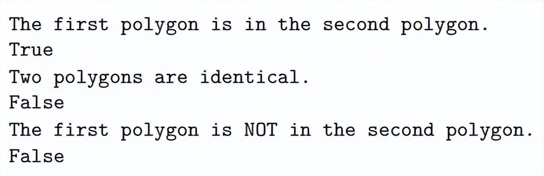
测试数据:
# Test
print(isin_polygon([Point(0.1,0.1),Point(0.2,0.2),Point(0.1,0.2),Point(0.1,0.1)],
                   [Point(0,0),Point(0,1),Point(1,1),Point(1,0),Point(0,0)]))
print(isin_polygon(multipolygons[29][0], multipolygons[29][0]))
print(isin_polygon(multipolygons[29][0], multipolygons[29][1]))
借助上面的 isin_polygon 函数,我们可以推导除组合多边形的质心。如我前面所述,组合多边形的中心就是多边形集合的面积加权平均值。
在函数中,我不仅考虑了一个多边形在另一个多边形中的情况,其中内多边形应该是一个负区域来表示另一个区域,例如梵蒂冈城应该被排除在罗马城中,因为它不属于意大利,因此我们可以预期罗马的数据将是组合多边形。我们可以把这看作是“正”区域中的“负”区域。
我还考虑了这样一种情况:一个区域位于一个更大的区域中,但中间的区域不应该包括在内。我们可以把它看作是一个“正”区域在一个“负”区域中,并且同时在的一个“正”区域,或者是另一个多边形中的一个多边形,这个多边形在一个更大的多边形中,应该属于第一个最小多边形的同一区域。该函数可以处理与此类似的更复杂的情况。这里的关键是:在组合多边形系统中,如果一个多边形在 n 个其他多边形中,并且 n 是奇数,那么这个小多边形的面积值应该是负的。否则,它应该为正值,这与上面的第二点类似。
def centroid_multipolygon(multipolygon):
"""
    该函数将返回组合多边形的面积和质心,并且包含多个多边形。

    INPUT:
    multipolygon: 组合多边形列表

    OUTPUT:
    组合多边形的面积和质心
    """

    # 初始化一个列表来记录每个多边形的面积和质心
    areas = []
    centers = []

for polygon in multipolygon:

# 得到每个多边形的面积和中心
        area, center = centroid(polygon)
        centers.append(center)

# 检查该多边形是否在另一个多边形中
        # 并相应地追加正负区域
        isinother = []
for other_poly in multipolygon:
            isinother.append(isin_polygon(polygon, other_poly, verbose=False))

if True in isinother and sum(isinother) % 2 == 1:
# 如果该多边形在其他多边形中是奇数个,那它应该是负的
            areas.append(-area)
else:
# 其他的所有情况,它应该是正的
            areas.append(area)

if len(centers) == 2:
# 如果只有两个多边形,中心将是连接两个中心点的直线上的加权点。
        sum_area = sum(areas)
        areas_proportion = [a / sum_area for a in areas]
        center_x = centers[0].x * areas_proportion[0] + \
                   centers[1].x * areas_proportion[1]
        center_y = centers[0].y * areas_proportion[0] + \
                   centers[1].y * areas_proportion[1]
        center_ = Point(center_x, center_y)

elif len(centers) > 2:
# 如果是组合多边形中有多个的多边形,则组合多边形的中心点将是所有多边形的中心点。
        centers.append(centers[0])
        area_, center_ = centroid(centers)

return sum(areas), center_
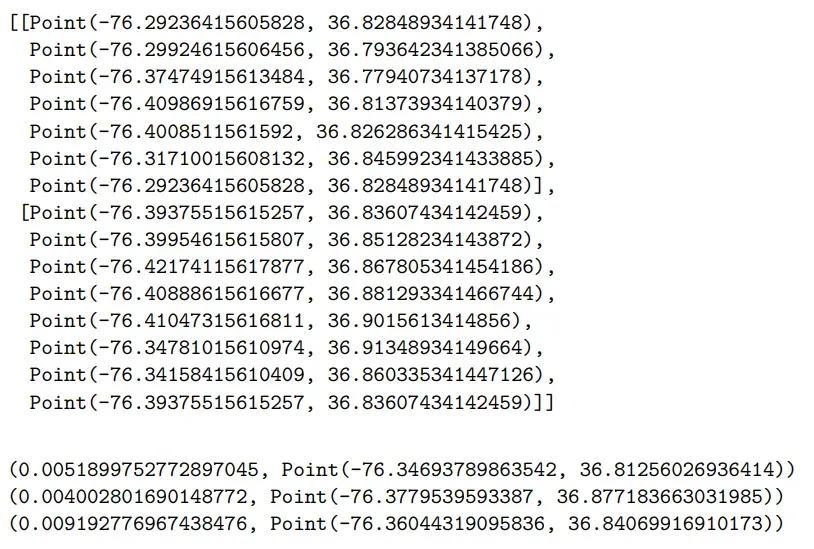
测试数据
# Test
display(multipolygons[36])
print(centroid(multipolygons[36][0]))
print(centroid(multipolygons[36][1]))
print(centroid_multipolygon(multipolygons[36]))
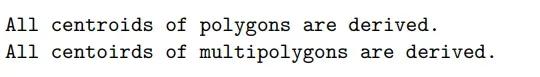
如果之前所有代码是正确的。下面的函数将获得所有多边形和组合多边形的质心。
def get_centroids(polygons, multipolygons):
"""
    该函数将导出所有多边形和组合多边形的所有质心。
    INPUT:
    polygons: 一个列表包含所有多边形
    multipolygons: 一个列表包含所有组合多边形
    OUTPUT:
    center_poly: 一个列表包含所有多边形的质心
    center_multipoly: 一个列表包含所有组合多边形的质心
    """

    # 初始化
    center_poly = []
    center_multipoly = []

# 用geom中质心函数得到所有多边形的质心
    for polygon in polygons:
        area, center = centroid(polygon)
        center_poly.append(center)
print('All centroids of polygons are derived.')

# 利用我们开发的函数得到所有组合多边形的质心
    for multip in multipolygons:
        area, center = centroid_multipolygon(multip)
# print(center)
        center_multipoly.append(center)
print('All centoirds of multipolygons are derived.')

return center_poly, center_multipoly

center_poly, center_multipoly = get_centroids(polygons, multipolygons)
4. 绘制地图和点符号
首先,我们可以通过之前计算的最小和最大坐标为地图定义一个合理的边界。
def get_plot_boundary(x_min, x_max, y_min, y_max):
"""
    此函数缩放图中轴极限的最小和最大坐标
    这是一个可选函数
    """
    x_min_ = round(x_min * 0.95) if x_min > 0 else round(x_min * 1.05)
    x_max_ = round(x_max * 1.05) if x_max > 0 else round(x_max * 0.95)
    y_min_ = round(y_min * 0.95) if y_min > 0 else round(y_min * 1.05)
    y_max_ = round(y_max * 1.05) if y_max > 0 else round(y_max * 1.05)
return x_min_, x_max_, y_min_, y_max_
x_min_, x_max_, y_min_, y_max_ = get_plot_boundary(x_min, x_max, y_min, y_max)
然后我们可以使用下面的函数来得到我们想到的图形。该函数将首先绘制从函数 get_coordinates_features 中提取的所有多边形和组合多边形。然后它将在每个质心上逐个绘制出圆形形状,其大小为我们从 attribute_scaling 中导出的比例缩放属性。我们增加了一些灵活性包括可选择颜色、透明度、自定义属性等。
在下面的绘制图函数中,有一个参数 reverse 将指向这一点:
它遵循我们在函数 centroid_multipolygon 中相似的逻辑,其中,如果在一个组合多边形系统中,一个多边形在另一个多边形中,其面积应该为负,以表示一个不属于更大的多边形的区域。在这里,这样一个多边形的点应该遵循与正常多边形相反的顺序,以便 Path 对象可以识别并雕刻出内部多边形。
但是在我们的数据中并没有这样的情况,我们目前也没有数据去测试组合多边形中的内多边形是否存在已经被反转的点了。如果是这样,那么我们就不应该再把点颠倒了。但为了保存灵活性,以防数据不能解决该问题,我们将此参数默认值设置为 False ,以不反转任何内容。
def point_symbol_map(polygons, multipolygons,
                     center_poly, center_multipoly,
                     attribute_poly, attribute_multipoly,
                     attribute_low=None, attribute_high=None,
                     reversed=False,
                     x_min=None, x_max=None, y_min=None, y_max=None,
                     figsize=(15, 9), tick_size=5,
                     edgecolor_map='black', facecolor_map='#ECECEC',
                     alpha_map=0.25, alpha_circle=0.5, alpha_grid=0.5,
                     attribute_color='blue', verbose=True):
"""
    此函数可以使点符号映射。
    INPUT:
    polygons: 多边形列表
    multipolygons: 组合多边形列表
    center_poly: 多边形的质心列表
    center_multipoly: 组合多边形的质心列表
    attribute_poly: 多边形的属性列表
    attribute_multipoly: 组合多边形的属性列表
    attribute_low: 要绘制的属性的下边界
    attribute_high: 要绘制的属性的下边界
    reversed: 是否反转内多边形(取决于数据)
    x_min: x轴的最小值
    x_max: x轴的最大值
    y_min: y轴的最小值
    y_max: y轴的最大值
    figsize: 图形的大小,应该是一个元组
    tick_size: 轴的刻度大小
    edgecolor_map: 映射的边缘颜色
    facecolor_map: 映射的表面颜色
    alpha_map: 映射的透明度
    alpha_circle: 点符号的透明度
    alpha_grid: 网格线的透明度
    attribute_color: 点符号的颜色
    verbose: 是否打印信息

    OUTPUT:
    没有,但是会有地图
    """

    _, ax = plt.subplots(figsize=figsize)

# 初始化要添加到Path对象的点
    multiverts = []
    multicodes = []

# 在多边形和组合多边形中逐个添加点
    for polygon in polygons:
        verts = [[p.x, p.y] for p in polygon]
        codes = [2 for p in polygon]
        codes[0] = 1  # code 1 暗示一个新的起点
        multiverts += verts
        multicodes += codes

for multipolygon in multipolygons:
for polygon in multipolygon:

# 我们是否需要颠倒内部的顺序?
            if reversed == True:
"""
                检查该多边形是否在另一个多边形中,
                如果该多边形表示一个负区域,那么在创建Path对象之前,需要将其顺序反转为与正常多边形不同的顺序。
                我没有其他文件来测试,如果多边形已经被颠倒了来表示负区域,那么它不应该再次被反转
                """
                isinother = []
for other_poly in multipolygon:
                    isinother.append(isin_polygon(polygon, other_poly, verbose=False))
if True in isinother and sum(isinother) % 2 == 1:
# 如果这个多边形在其他多边形里为奇数个,那它应该颠倒过来
                    polygon.reverse()
            verts = [[p.x, p.y] for p in polygon]
            codes = [2 for p in polygon]
            codes[0] = 1
            multiverts += verts
            multicodes += codes

# 创建Path对象并绘制它。
    # zorder = 0 确保它将被放回zorder = 1 的散射体下
    path = Path(multiverts, multicodes)
    patch = PathPatch(path, edgecolor=edgecolor_map, facecolor=facecolor_map, alpha=alpha_map, zorder=0)
    ax.add_patch(patch)
if verbose:
print("Polygons drawed.")

# 在每个区域的中心绘制圆形符号,大小为多边形和组合多边形的比例缩放属性
    for center, attr in zip(center_poly, attribute_poly):
if attribute_low is not None and attribute_high is not None:
if attr >= attribute_low and attr <= attribute_high:
                ax.scatter(center.x, center.y, s=attr, c=attribute_color, alpha=alpha_circle, zorder=1)
elif attribute_low is not None:
if attr >= attribute_low:
                    ax.scatter(center.x, center.y, s=attr, c=attribute_color, alpha=alpha_circle, zorder=1)
elif attribute_high is not None:
if attr <= attr <= attribute_high:
                    ax.scatter(center.x, center.y, s=attr, c=attribute_color, alpha=alpha_circle, zorder=1)
else:
                ax.scatter(center.x, center.y, s=attr, c=attribute_color, alpha=alpha_circle, zorder=1)

for center, attr in zip(center_multipoly, attribute_multipoly):
if attribute_low is not None and attribute_high is not None:
if attribute_low <= attr <= attribute_high:
                ax.scatter(center.x, center.y, s=attr, c=attribute_color, alpha=alpha_circle, zorder=1)
elif attribute_low is not None:
if attr >= attribute_low:
                ax.scatter(center.x, center.y, s=attr, c=attribute_color, alpha=alpha_circle, zorder=1)
elif attribute_high is not None:
if attr <= attr <= attribute_high:
                ax.scatter(center.x, center.y, s=attr, c=attribute_color, alpha=alpha_circle, zorder=1)
else:
            ax.scatter(center.x, center.y, s=attr, c=attribute_color, alpha=alpha_circle, zorder=1)

if verbose:
print("Attribute points drawed.")

# 创建轴刻度
    x_ticks = np.arange(-360, 361, tick_size)
    y_ticks = np.arange(-90, 91, tick_size)

# 添加网格线
    ax.grid(which='major', alpha=alpha_grid)

# 指定轴的最小-最大边界
    if (x_min is not None and
            x_max is not None and
            y_min is not None and
            y_max is not None):
        ax.set_xlim(x_min, x_max)
        ax.set_ylim(y_min, y_max)

# 将刻度和轴设置为相等,以避免失真
    ax.set_xticks(x_ticks)
    ax.set_yticks(y_ticks)
    ax.axis('equal')
    plt.show()

point_symbol_map(polygons, multipolygons,
                 center_poly, center_multipoly,
                 attribute_poly_a, attribute_multipoly_a,
                 figsize=(15,9), tick_size=5,
                 edgecolor_map='black', facecolor_map='#ECECEC',
                 alpha_map=0.5, alpha_circle=0.5, alpha_grid=0.5,
                 attribute_color='blue', verbose=True)
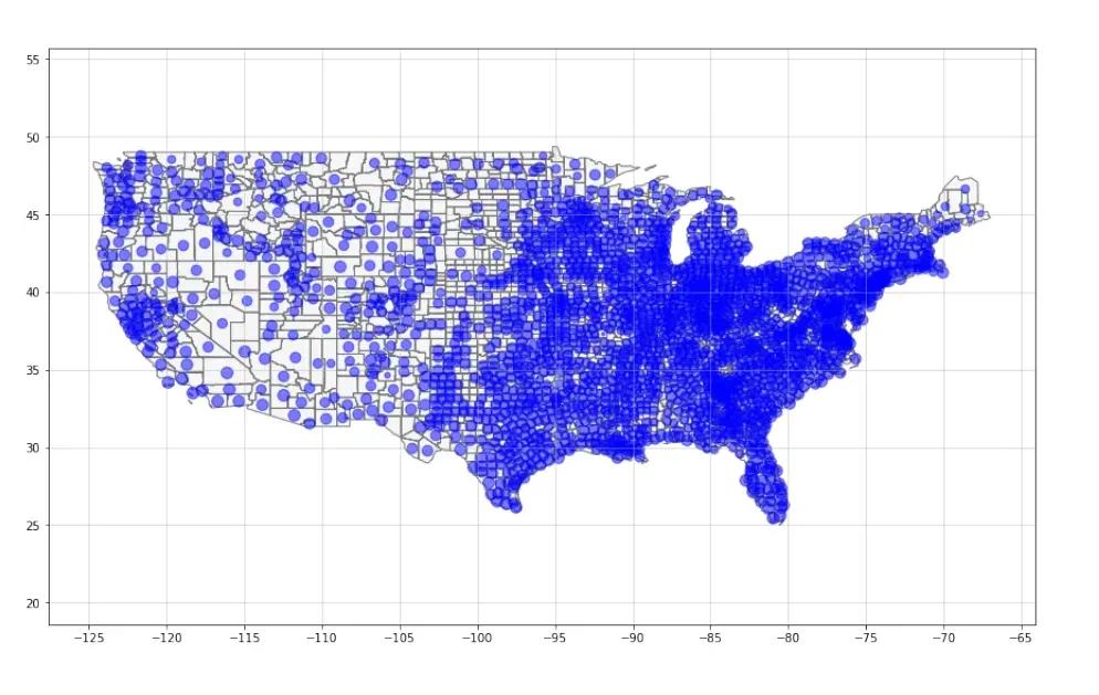
我们可以看到,正如我们讨论的那样,圆圈的大小差别不大,因为就其属数值而言,属性的差异太小了。因此,我们将使用插值转换的数据再次测试不同的颜色,透明度-也是为了演示功能
point_symbol_map(polygons, multipolygons,
                 center_poly, center_multipoly,
                 attribute_poly_i, attribute_multipoly_i,
                 figsize=(15,9), tick_size=2.5,
                 edgecolor_map='darkblue', facecolor_map='grey',
                 alpha_map=0.3, alpha_circle=0.4, alpha_grid=0.5,
                 attribute_color='red', verbose=True)
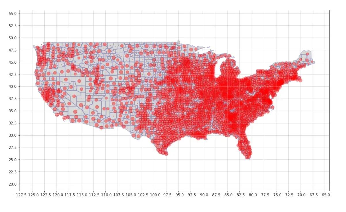
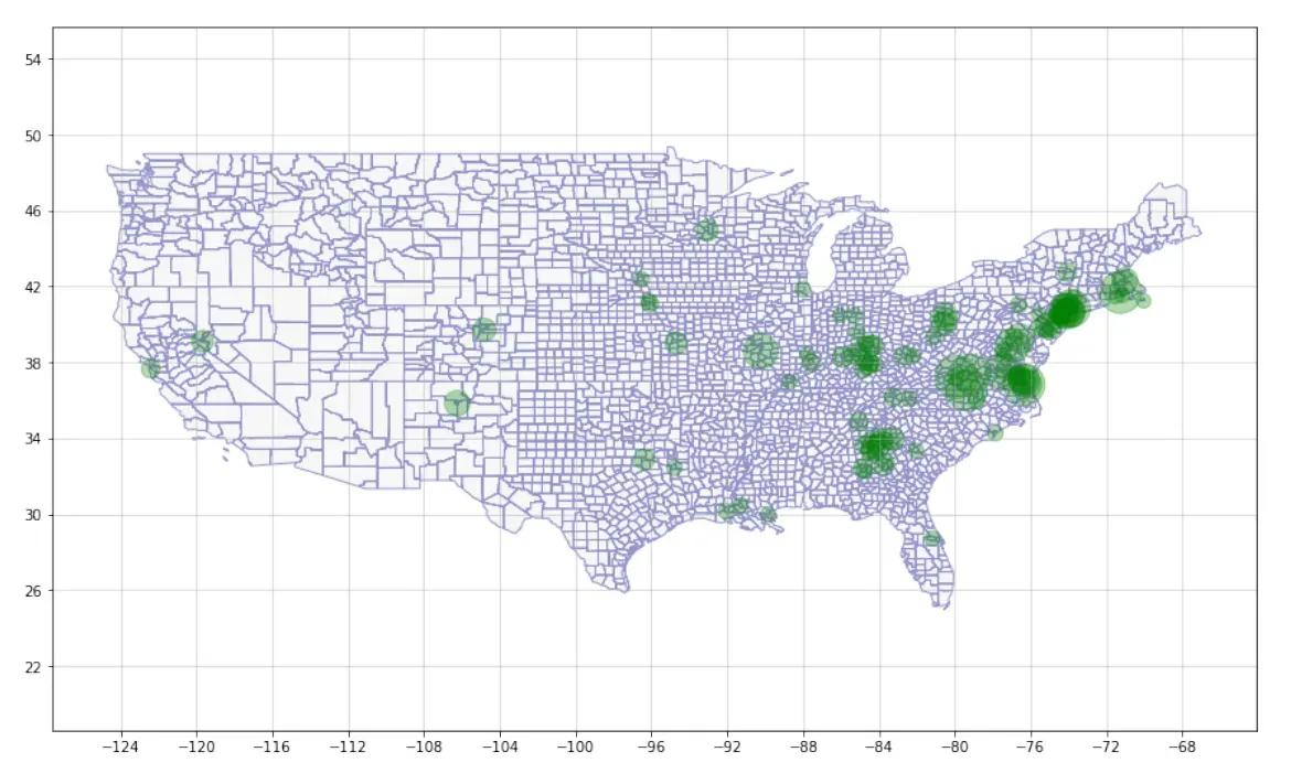
这张地图上尺寸的差异更明显,因为尺寸是“拉长的”。我们可以很容易地看到,美国东部和西海岸的城市人口较多。然后让我们尝试使用自定义属性。我们用城市人口除以面积得到每平方公里的城市人口。同样,我们使用插值方法,因为我们可能想看到不同的地方。
attribute_poly_new = []
attribute_multipoly_new = []
for i in range(len(mapdata)):
city = mapdata[i]['properties']['NAME']
state = mapdata[i]['properties']['STATE_NAME']

if mapdata[i]['geometry']['type'].lower() == 'polygon':
try:
            attr = mapdata[i]['properties']['UrbanPop']/mapdata[i]['properties']['AreaKM2']
            attribute_poly_new.append(attr)
except:
#  636,没有AreaKM2,没有UrbanPop,全是0
            attribute_poly_new.append(0)

elif mapdata[i]['geometry']['type'].lower() == 'multipolygon':
try:
            attr = mapdata[i]['properties']['UrbanPop']/mapdata[i]['properties']['AreaKM2']
            attribute_multipoly_new.append(attr)
except:
            attribute_multipoly_new.append(0)
attribute_poly_upk, attribute_multipoly_upk = attribute_scaling(attribute_poly_new,
                                                                attribute_multipoly_new, max_radius=1000,
                                                                min_radius=1, scale='interpolated')
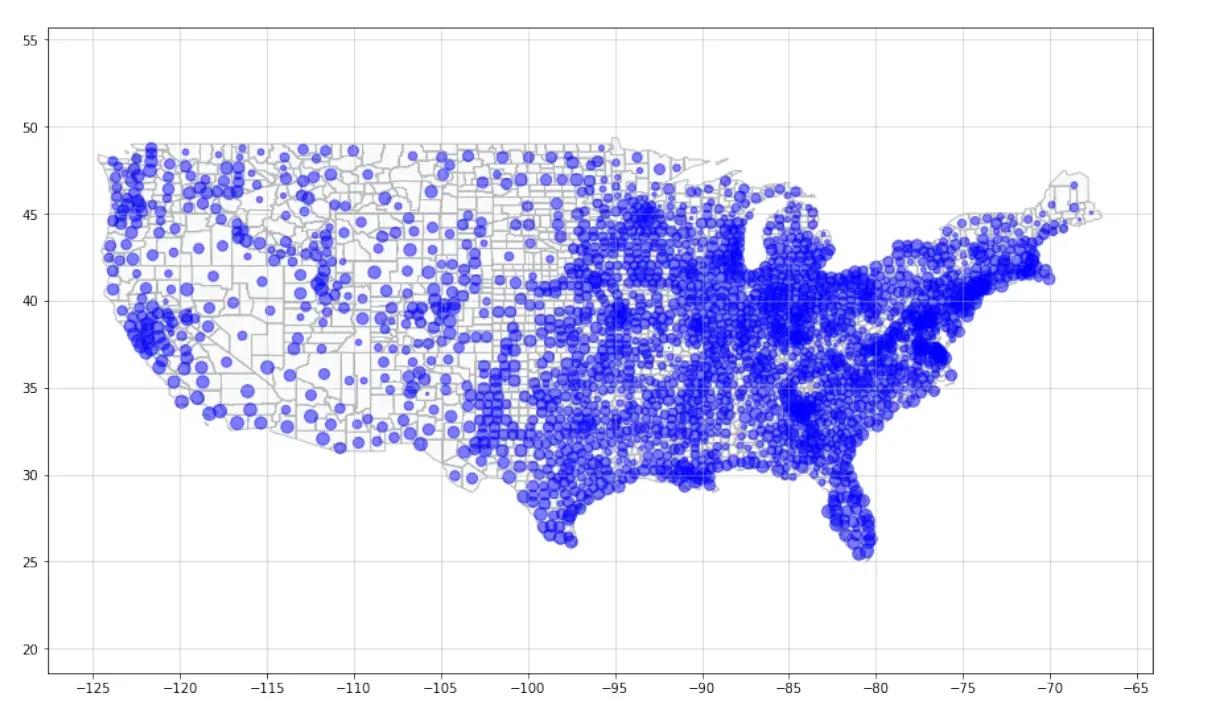
应用内插缩放比例:从 1 到 1000。
point_symbol_map(polygons, multipolygons,
                 center_poly, center_multipoly,
                 attribute_poly_upk, attribute_multipoly_upk,
                 tick_size=4,
                 edgecolor_map='darkblue', facecolor_map='#ECECEC',
                 alpha_map=0.4, alpha_circle=0.3, alpha_grid=0.5,
                 attribute_color='green')
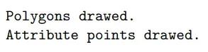
这一点在美国城市人口较多的地方表现得更为明显。现在让我们来看看城市人口密度最高的 10 个县。
# 我们将所有属性组合起来,对它们进行排序,得到前10名
all_upk = attribute_poly_upk + attribute_multipoly_upk
all_upk.sort(reverse=True)
boundary_top10 = min(all_upk[:10])
print(boundary_top10)
492.88759882214583
point_symbol_map(polygons, multipolygons,
                 center_poly, center_multipoly,
                 attribute_poly_upk, attribute_multipoly_upk,
                 attribute_low=boundary_top10, tick_size=4,
                 edgecolor_map='darkblue', facecolor_map='#ECECEC',
                 alpha_map=0.4, alpha_circle=0.3, alpha_grid=0.5,
                 attribute_color='green')
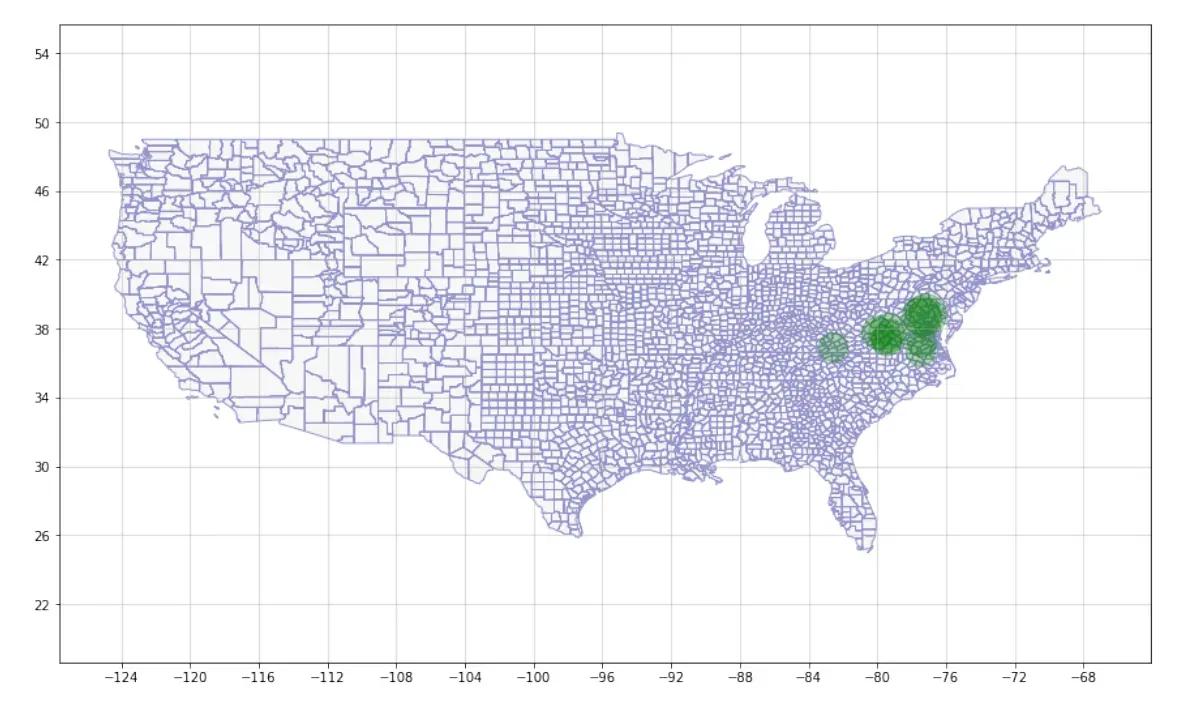
我们可以看到东部的城市人口密度最高。最大的圆圈似乎在纽约市。那其他地区呢?
我们现在使用一个简单的乘数将属性从每平方公米的城市人口放大到每 1000 平方米的城市人口,乘数为 1000。然后我们将绘制那些区域的数值小于 10 的地区,这意味着每 1000 平方公里的城市人口小于 10 人。
attribute_poly_m, attribute_multipoly_m = attribute_scaling(attribute_poly_new,
                                                            attribute_multipoly_new, max_radius=1000,
                                                            multiplier=1000,scale = 'multiplier')
应用 Multiplier scaling : 1000x
point_symbol_map(polygons, multipolygons,
                 center_poly, center_multipoly,
                 attribute_poly_m, attribute_multipoly_m,
                 attribute_high=10, tick_size=4,
                 edgecolor_map='darkblue', facecolor_map='#ECECEC',
                 alpha_map=0.4, alpha_circle=0.3, alpha_grid=0.5,
                 attribute_color='green')
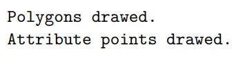
我们可以在地图上看到很多小绿点,这表明城市人均人口比例很低。下面的图表显示了每平方米城市人口在 0.1 到 1 之间的地区。 它很好地说明了我们的 filter 函数在绘图中的作用。
point_symbol_map(polygons, multipolygons,
                 center_poly, center_multipoly,
                 attribute_poly_m, attribute_multipoly_m,
                 attribute_low=100, attribute_high=1000,
                 tick_size=4,
                 edgecolor_map = 'darkblue', facecolor_map = '#ECECEC',
                 alpha_map = 0.4, alpha_circle = 0.3, alpha_grid = 0.5,
                 attribute_color = 'green')
5. 手册-如何使用模块
上面我已经演示了这个项目的几乎所有功能,并在代码中解释了许多细节,但我将在这里再次总结。 请按以下步骤使用此模块:
- 在 dictionary / JSON 中准备至少包含以下键的 shape 数据:
- 使用函数get_coordinates_features()来提取区域/多边形的坐标,也可以提取字典中的特征。
- 如果你想自定义特征,请按顺序排序,顺序与对应多边形的顺序相同。你可以使用带有 location 和相应属性值的字典来与函数 get_coordinates_features()返回的区域变量来相匹配。这样,按所需的顺序对属性进行排序就不难了。
- 使用attribute_scaling()函数来缩放属性,以避免在最终的图表上出现过大或过小的圆圈。
- 使用函数get_centroids()来查找所有多边形和组合多边形的质心。它们将是最终地图上属性的圆心。
- 使用函数point_symbol_map()和函数中引入的参数来获得所需颜色的地图图表。
或者,步骤 2 到 6 被压缩到plot_attributes() 下面的函数中,一些参数是默认的。 你可以简单地使用 mapdata 和 mapdata 字典中的 attribute 键来调用该函数,以绘制点符号映射。这里给出了一个示例:
def plot_attributes(mapdata, attribute, verbose=False,
                    max_radius=100, min_radius=1, multiplier=100, scale='abosolut',
                    attribute_low=None, attribute_high=None,
                    reversed=False, figsize=(15, 9), tick_size=5,
                    edgecolor_map='black', facecolor_map='#ECECEC',
                    alpha_map=0.25, alpha_circle=0.5, alpha_grid=0.5,
                    attribute_color='blue'
                    ):
    polygons, multipolygons, attribute_poly, attribute_multipoly, \
        _, _, _, _, _ = get_coordinates_features(mapdata=mapdata,
                                                 attribute=attribute,
                                                 verbose=verbose)

    attribute_poly_, attribute_multipoly_ = attribute_scaling(attribute_poly,
                                                              attribute_multipoly,
                                                              max_radius=max_radius, min_radius=min_radius, scale=scale)

    center_poly, center_multipoly = get_centroids(polygons, multipolygons)
    point_symbol_map(polygons, multipolygons,
                     center_poly, center_multipoly,
                     attribute_poly_, attribute_multipoly_,
                     attribute_low=attribute_low, attribute_high=attribute_high,
                     reversed=reversed,
                     figsize=figsize, tick_size=tick_size,
                     edgecolor_map=edgecolor_map, facecolor_map=facecolor_map,
                     alpha_map=alpha_map, alpha_circle=alpha_circle,
                     alpha_grid=alpha_grid,
                     attribute_color=attribute_color, verbose=verbose)
    plot_attributes(mapdata, 'UrbanPop')
6. 附录
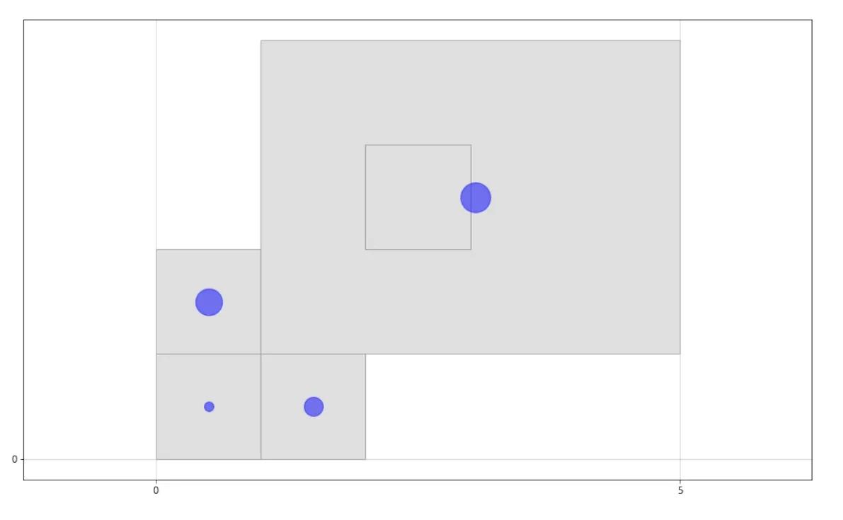
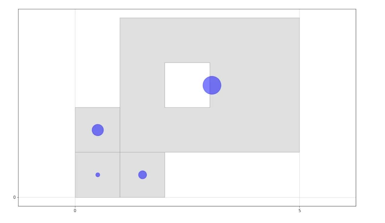
在本部分中,我们将解决“一个多边形位于另一个多边形中”的问题。下面两张图展示了演示:
我们有其中一个多边形在另一个多边形中这种数据,但内多边形的点的顺序实际上应该是相反的。使用 reversed=True 参数或 reversed=False 参数调用函数 point_symbol_map()两次。我们可以看出其中的差别。因此,这个参数可以给我们更多的取决于数据的灵活性。
pls = [[Point(0, 0), Point(0, 1), Point(1, 1), Point(1, 0), Point(0, 0)],
       [Point(1, 0), Point(1, 1), Point(2, 1), Point(2, 0), Point(1, 0)],
       [Point(0, 1), Point(0, 2), Point(1, 2), Point(1, 1), Point(0, 1)]]
mpls = [[[Point(1, 1), Point(1, 4), Point(5, 4), Point(5, 1), Point(1, 1)],
         [Point(2, 2), Point(2, 3), Point(3, 3), Point(3, 2), Point(2, 2)]]]
attpl = [100, 400, 800]
attmpl = [2000]
center_pl, center_mpl = get_centroids(pls, mpls)
point_symbol_map(pls, mpls, center_pl, center_mpl, attpl, attmpl,
                 facecolor_map='grey', reversed=True)
pls = [[Point(0, 0), Point(0, 1), Point(1, 1), Point(1, 0), Point(0, 0)],
       [Point(1, 0), Point(1, 1), Point(2, 1), Point(2, 0), Point(1, 0)],
       [Point(0, 1), Point(0, 2), Point(1, 2), Point(1, 1), Point(0, 1)]]
mpls = [[[Point(1, 1), Point(1, 4), Point(5, 4), Point(5, 1), Point(1, 1)],
         [Point(2, 2), Point(2, 3), Point(3, 3), Point(3, 2), Point(2, 2)]]]
attpl = [100, 400, 800]
attmpl = [1000]
center_pl, center_mpl = get_centroids(pls, mpls)
point_symbol_map(pls, mpls, center_pl, center_mpl, attpl, attmpl,
                 facecolor_map='grey', reversed=False)